Twenty years ago, I presented a study at THIESEL 2006 that challenged two assumptions then common in industrial CFD: that high-Reynolds-number wall functions were adequate for predicting diesel intake-port flow, and that a stationary geometry could reasonably be treated as a steady-flow problem.
The results suggested otherwise — but for two distinct reasons.
Resolving the near-wall flow changed the predicted separation and corrected a mass-flow error of around 12%. Further, the modified separated jet direction and strength changed substantially the swirl of the flow developing in the cylinder.
At the same time, calculations using conventional wall-function treatment were proving difficult to converge to a steady solution. The improved near-wall cases also failed to converge to a steady solution.
Restarting from the unconverged steady flow field and solving transiently suggested that this behaviour was revealing something physical: the stationary intake-port geometry, under steady imposed boundary conditions, was generating large-scale unsteady flow structures and instabilities that could not be represented by the assumed steady-state approach.
Improved near-wall treatment was therefore required to predict the mean flow correctly, while transient simulation was required to expose important dynamics of that flow.
The non-converging steady calculation was already trying to tell us that something was wrong with the assumption of steadiness. The industrial instinct was to regard failure to converge as a numerical problem to be suppressed. However once the calculation was allowed to evolve in time, some of that apparent numerical difficulty emerged as physical flow instability.
Allowing the flow to be unsteady did not, by itself, make the CFD predictive. The physics responsible for determining the flow still had to be modelled correctly — and in this case much of that physics originated at the wall.
Twenty years later, computing power is enormously greater. So where have we spent it? Are important flow physics still being hidden behind long-held assumptions in our CFD methods?
What we found in 2006
Two substantially different intake-port geometries were investigated in the original study: a heavy-duty 125 mm-bore engine with siamese inlet ports (Case A), and a light-duty 96 mm-bore engine with separate dual inlet ports (Case B). Two valve lifts were examined for each geometry. Much of the discussion below focuses on Case B, where the interaction between the two port flows and their sensitivity to near-wall treatment became particularly revealing.
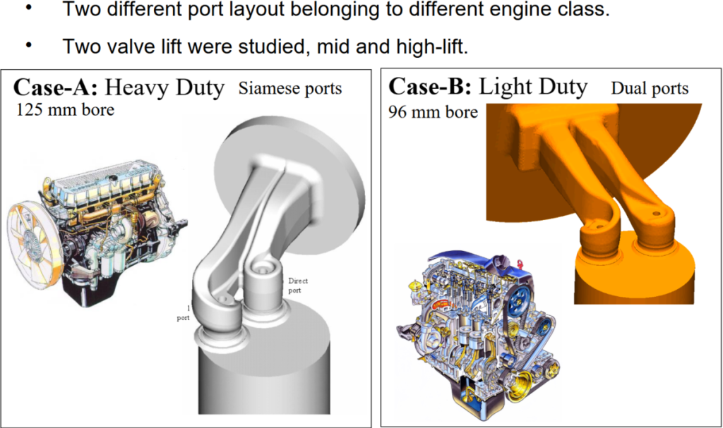
Intake-port geometries investigated in the THIESEL 2006 study. Case A represents a 125 mm-bore heavy-duty engine with siamese inlet ports; Case B a 96 mm-bore light-duty engine with separate dual ports. The later examples of valve-stem wake behaviour, jet interaction and upstream boundary-layer sensitivity are principally drawn from Case B.
The stationary-flow simulations reproduced the basic arrangement of the experimental flow rig. A pressure difference was imposed between the upstream plenum and the outlet of an extended dummy cylinder, drawing air through the stationary inlet ports and valves in the same manner as the experimental flow rig.
Global quantities used for validation included mass flow and the angular-momentum flux evaluated at the equivalent torquemeter location downstream of the cylinder head.
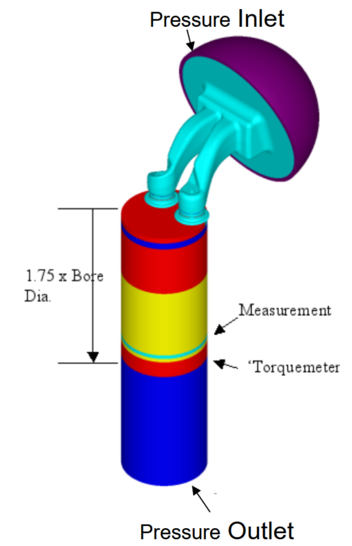
Can the numerical method conserve swirl?
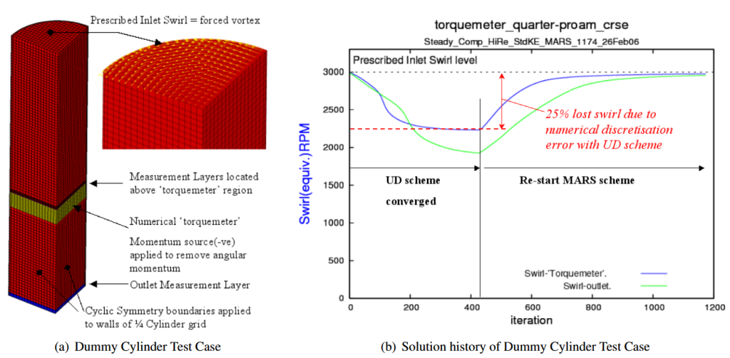
Before investigating the more complicated behaviour of the intake-port flow, we performed a deliberately simple numerical test. A prescribed swirling velocity field was imposed at the inlet of a straight cylindrical domain, representing in simplified form the swirl entering the dummy cylinder beneath an intake port on a stationary flow rig.
The purpose was not to model an intake port, but to ask a much more fundamental question: once angular momentum has been introduced into the computational domain, can the numerical method transport it correctly?
The cylinder wall was deliberately specified as a slip boundary, eliminating wall shear and therefore removing any physical mechanism by which angular momentum could be lost from the flow. The angular-momentum flux should consequently remain constant through successive axial sections of the cylinder. Any reduction in the imposed swirl could therefore be attributed directly to numerical discretisation error, providing a simple conservation test of the numerical scheme.
The result was striking. With the first-order upwind differencing (UD) scheme then commonly used for industrial intake-port CFD, approximately 25% of the imposed angular momentum was lost numerically at a representative industrial mesh resolution. Increasing mesh resolution reduced the error, but the numerical diffusion remained substantial. Using the higher-order MARS discretisation scheme, by comparison, approximately 98% of the angular momentum was conserved.
In other words, a significant part of the predicted loss of swirl had nothing to do with viscosity, wall friction or the physics of the flow. It was being removed by the numerical discretisation itself.
The temptation of a robust turnkey process
First-order upwind nevertheless had one particularly attractive property: it was robust. Intake-port calculations which were difficult to converge using higher-order discretisation could often be persuaded to produce a steady solution using UD. But the conservation test illustrates the price of that robustness. The same numerical diffusion which dissipated angular momentum also damped velocity gradients and flow structures.
A calculation could therefore become easier to converge precisely because the numerical method was suppressing the behaviour which made the physical flow difficult to represent as steady.
Numerical robustness and physical fidelity are not the same thing.
At the time, the conventional industrial approach to intake-port CFD was a steady-state RANS calculation using high-Reynolds-number turbulence modelling and wall functions. The attraction was obvious: the method was robust, computationally affordable and capable of providing the global quantities used to assess port designs, particularly mass flow and swirl.But agreement in a global quantity does not necessarily mean that the underlying flow field is being predicted correctly. In our test cases, the conventional wall-function approach could produce apparently reasonable results for some geometries, while for another the predicted mass flow differed from experiment by approximately 12% and yet more significantly, the predicted swirl torque showed up to a factor x2 discrepancy, proving considerably more difficult to reproduce reliably and typically showed substantial fluctuations and a dogged resistance to converge to a stable value.
Resolving the near-wall flow around the valve seat changed the predicted boundary-layer separation and the direction and strength of the emerging valve-curtain jet. Yet the full explanation for discrepancy with experiment was not revealed as expected from the valve seat region alone.
A controlled two-dimensional axisymmetric test case isolated the influence of the near-wall treatment at the valve seat. Replacing the conventional high-Reynolds-number wall-function treatment locally with low-Reynolds-number resolution changed the predicted boundary-layer separation and consequently the mass flow through the valve curtain.
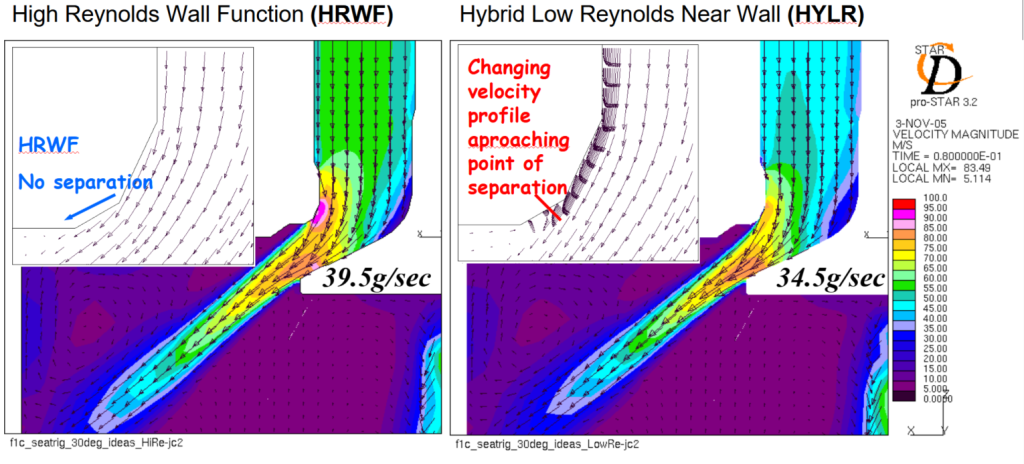
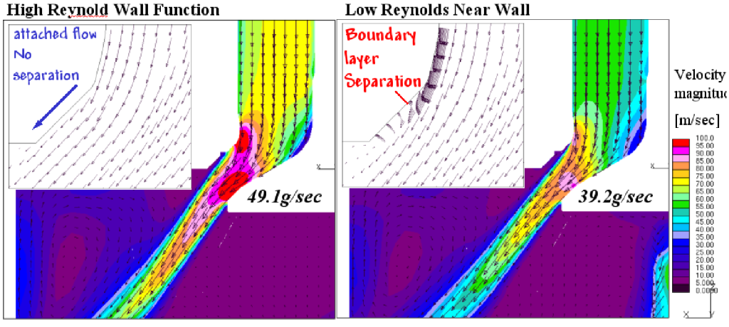
The influence of near-wall treatment in the complete three-dimensional intake port was considerably more complex than this isolated valve-seat example.
The global integral mass flow is only the first test. It tells us how much air passes through the port. Swirl is a considerably more demanding metric because it depends not only on how much air crosses the valve curtain, but where it crosses, its direction, momentum and moment arm about the cylinder axis. Errors which may partly disappear when the flow is integrated into a single mass-flow number can remain very significant when predicting angular momentum. With two inlet valves the problem becomes more complicated again. The valve jets interact within the cylinder. Even with stationary geometry and steady boundary conditions, there is no requirement for these separated jets, wakes and shear layers to remain steady—or even to preserve the apparent symmetry of the geometry.
Failure of a higher-order calculation to converge does not, by itself, prove that the underlying flow is unsteady. But neither should failure to converge automatically be regarded as a numerical defect to be cured by increasing numerical diffusion. In the intake-port calculations, running the problem transiently provided another explanation.
A stationary geometry does not imply a steady flow
This is easiest to see by stripping the problem back to one of the simplest examples in fluid mechanics: – a stationary cylinder in a steady cross-flow. Neither the geometry nor the imposed boundary conditions need change with time, yet above the appropriate Reynolds-number regime the wake is inherently unsteady. Vortices are shed alternately from either side of the cylinder, producing an oscillating wake. The unsteadiness belongs to the flow, not to the geometry.
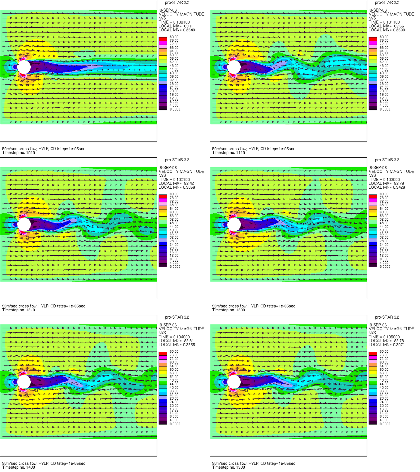
Transient URANS animation – calculation of 50 m/s cross-flow over a stationary cylinder. Despite stationary geometry and steady inlet conditions, the separated wake develops an inherently unsteady structure. Calculation from the original THIESEL 2006 study.
This canonical example is directly relevant to the intake-port geometry. Each valve stem presents a bluff body to the incoming port flow. The transient calculation shows the development of asymmetric structures around and downstream of the valve stems, analogous to the vortex-shedding behaviour demonstrated by the simple cylinder calculation.
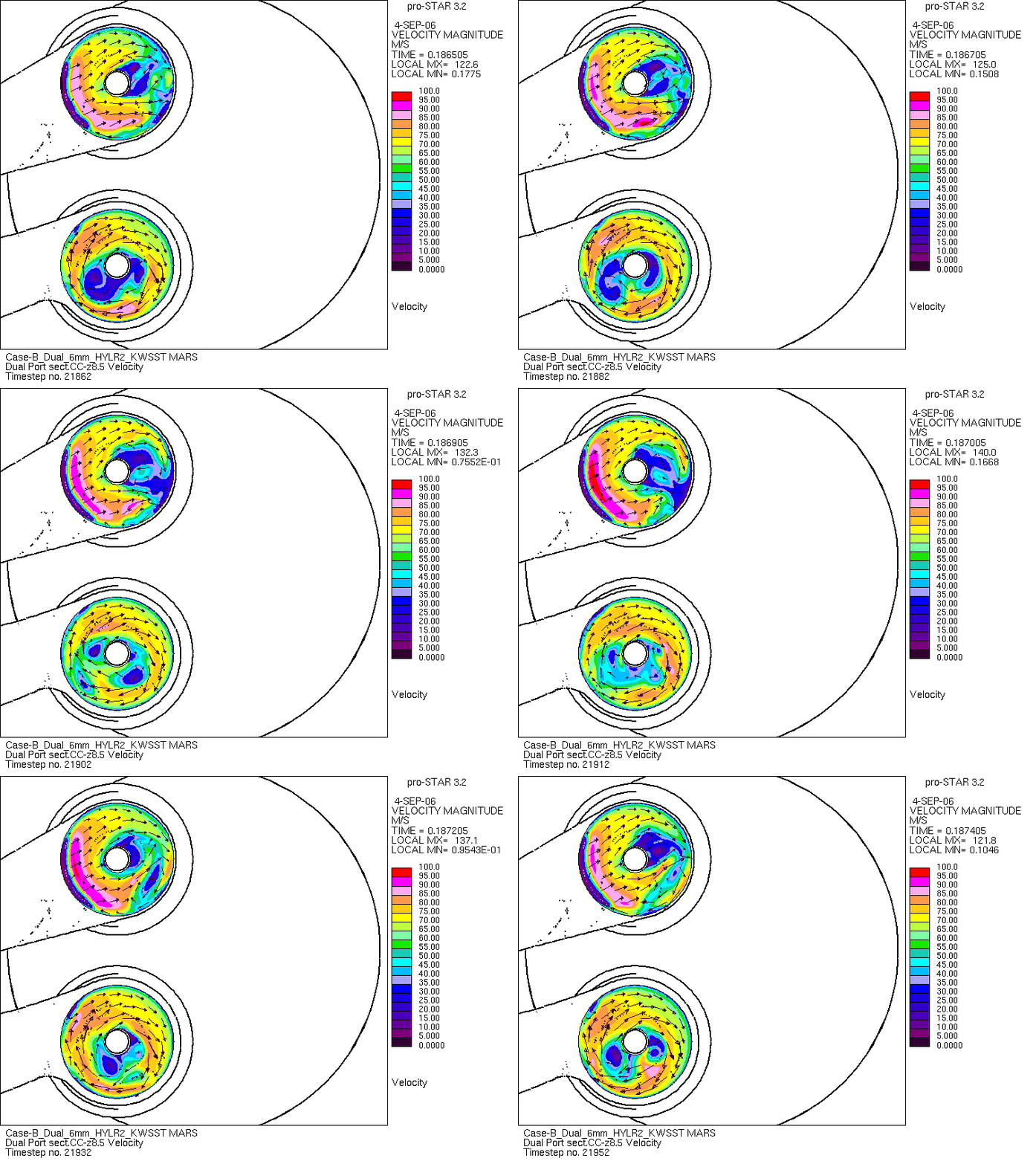
Transient URANS animation — Cross-flow around the inlet-valve stems. The instantaneous velocity field shows asymmetric wake structures developing behind the stationary valve stems, providing a direct connection between the canonical cylinder cross-flow example and the unsteady structures present within the intake port. From the THIESEL 2006 study.
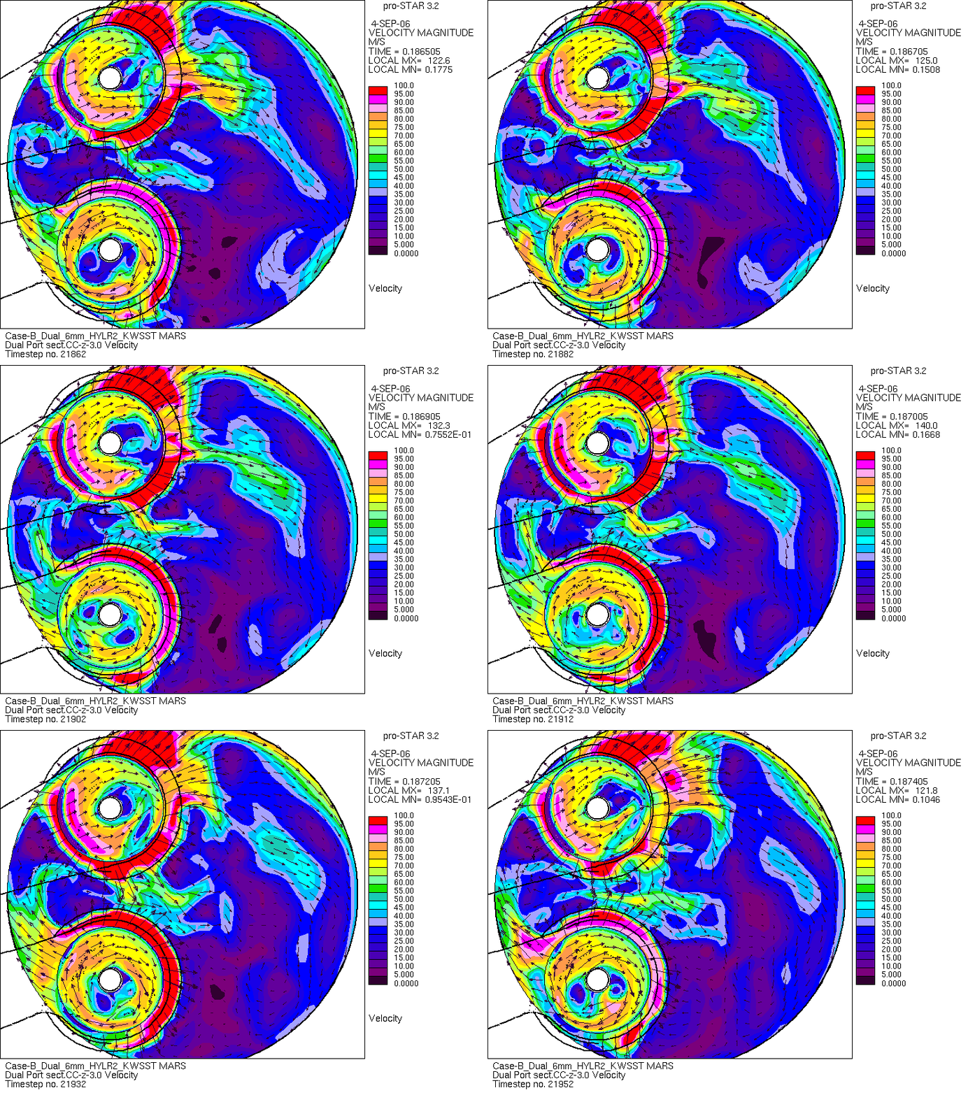
But the valve-stem wakes are only one source of unsteadiness. Downstream, the separated flows emerging through the two valve curtains form jets which interact with one another inside the cylinder.
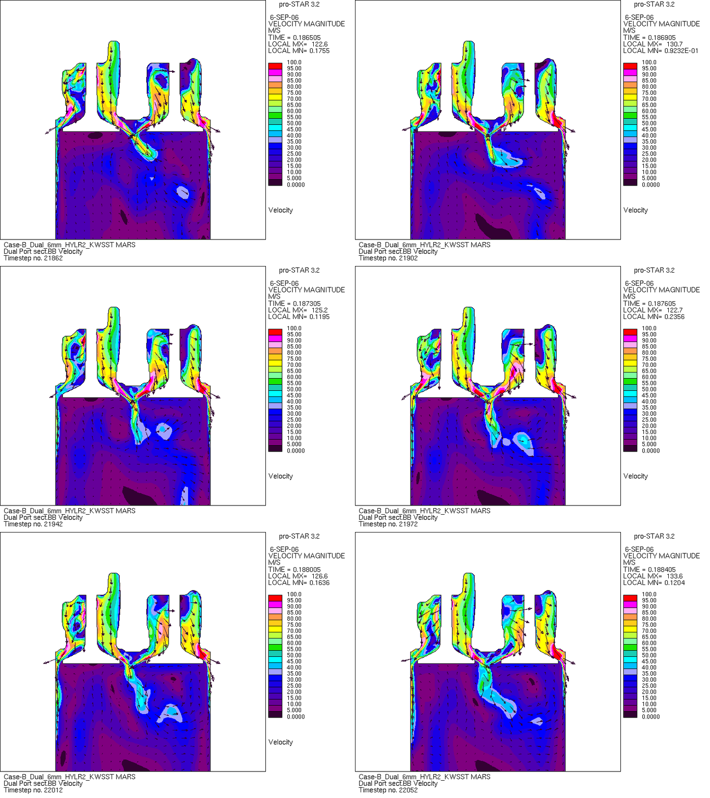
Transient URANS animation — Port-to-port interaction in the dual-inlet-valve calculation. The valve-curtain jets fluctuate in position and direction and interact as they enter the cylinder, illustrating the jet-flapping behaviour observed in the THIESEL 2006 study.
The instability was not where we expected.
The most revealing result, however, came from a less obvious part of the flow field. Attention had naturally been focused on the valve seat, valve curtain and the interaction of the two inlet jets. But extending the low-Reynolds-number treatment upstream exposed another important source of sensitivity: separation and reattachment along the upper wall, or roof, of the intake-port canal.
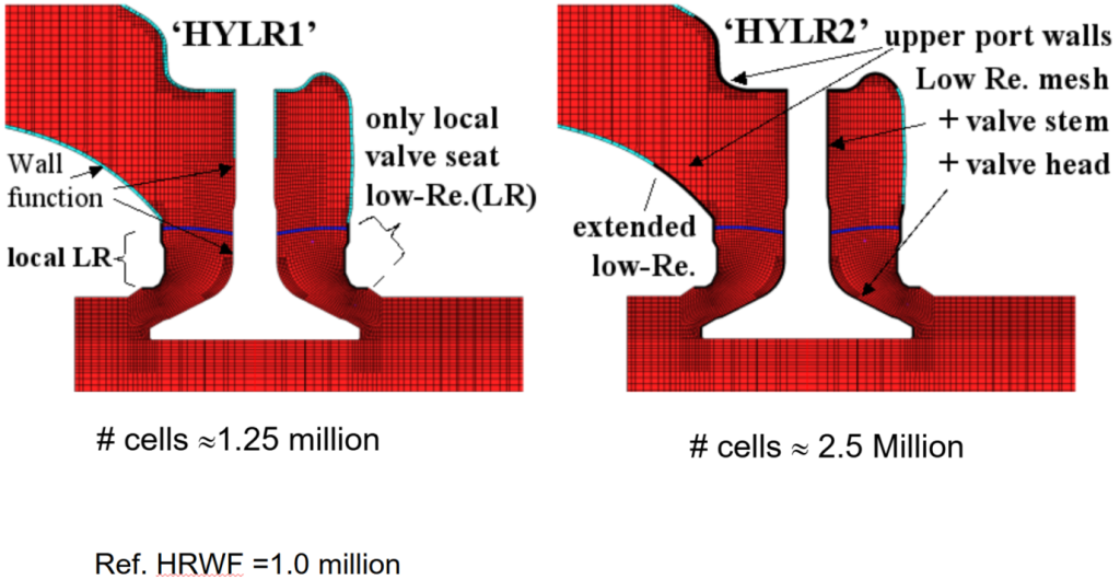
Resolving this region changed the flow delivered to the valve before it even reached the valve curtain. The position and behaviour of the separated region influenced the mass flow through the port, the direction and strength of the emerging valve jet and, consequently, the angular momentum subsequently developed within the cylinder.
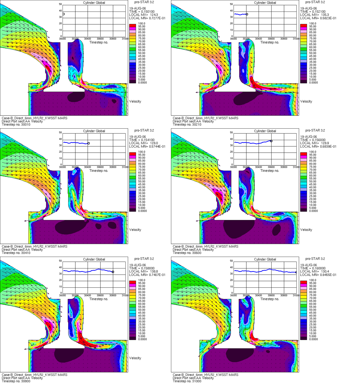
Transient URANS animation — Unsteady separation and reattachment on the upper wall of the intake port. Extending the low-Reynolds-number near-wall treatment upstream revealed an unexpectedly important source of variation in the flow delivered to the valve, affecting mass flow, valve-jet development and ultimately cylinder swirl. From the THIESEL 2006 study.
More importantly, the separation was itself unsteady. The transient calculation revealed movement of the separation and reattachment structure which propagated downstream into the valve flow. What could appear at the cylinder level as unstable swirl or interacting valve jets therefore had an upstream origin that was not obvious from the global quantities alone.
The discrepancy observed at the cylinder was therefore not necessarily generated in the cylinder. Its origin could lie upstream in boundary-layer behaviour that the conventional wall-function treatment was poorly equipped to predict.
The importance of the upstream boundary layer became particularly apparent in the Case-B 6 mm direct-port calculation. With the conventional high-Reynolds-number wall-function (HRWF) treatment, the predicted mass flow was approximately 12% above the experimental measurement, while the predicted swirl torque was more than twice the measured value.
Extending the locally resolved low-Reynolds-number treatment upstream along the port walls in the HYLR2 model substantially changed both predictions. The mass-flow prediction moved into close agreement with experiment and the large discrepancy in swirl torque was substantially reduced. The corresponding time-averaged velocity fields show that this was not simply a correction to the wall shear: changing the upstream boundary-layer treatment altered the flow subsequently delivered to the valve curtain and therefore the structure of the jet entering the cylinder.
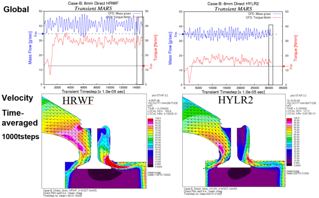
Effect of extended low-Reynolds-number near-wall treatment in the Case-B 6 mm direct port. The conventional HRWF calculation overpredicts measured mass flow by approximately 12% and swirl torque by more than a factor of two. Extending the low-Reynolds treatment upstream in HYLR2 substantially improves both global quantities and produces a markedly different time-averaged flow field approaching the valve and valve curtain. From the THIESEL 2006 presentation.
Mass flow tells us how much air got through. Swirl tells us much more about whether the calculation got the flow itself right.
Conclusion
A stationary flow-rig geometry therefore provides no physical justification for assuming that its flow field must possess a steady solution.
Failure to obtain a steady converged solution is not necessarily evidence of a numerical problem. It may be evidence that the assumed steady physical solution does not exist.
It should come as no surprise to a student of fluid dynamics that an internal-flow geometry with strong wall interactions can generate significant inherent unsteadiness at large, coherent scales. Such organised motion is distinct from the turbulent fluctuations represented statistically by the RANS turbulence model. Where separation, reattachment and vortex shedding are driven by near-wall flow, reliance upon the major simplifications inherent in wall-function modelling should therefore be questioned.
The use of URANS here raises a further question rather than providing a final answer. Internal flows of this kind can contain large-scale organised and coherent structures superimposed upon broadband turbulent motion. To what extent such structures can legitimately be resolved by URANS, rather than being entangled with the statistical assumptions of the turbulence closure, is itself a substantial modelling question.
More rigorous scale-resolving approaches such as LES offer an obvious route towards resolving a greater part of this unsteady flow physics, but introduce another fundamental difficulty: the enormous range of scales that must be bridged between the relatively inviscid core flow and the viscous-dominated near-wall region where separation and reattachment may originate.
That interface between the resolved outer flow and the viscous near-wall physics represents, in the terminology of this site, a “viscous limit” — the point at which a convenient modelling approximation encounters flow physics that it can no longer safely neglect.
This work was originally presented at the THIESEL 2006 Conference on Thermo- and Fluid Dynamic Processes in Diesel Engines. The original conference paper is available here: